通篇以iris(鸢尾花)数据集为例(下图为数据集部分内容)1.如何对其进行数据处理?从iris数据集中,提取前两个分类的数据,并...

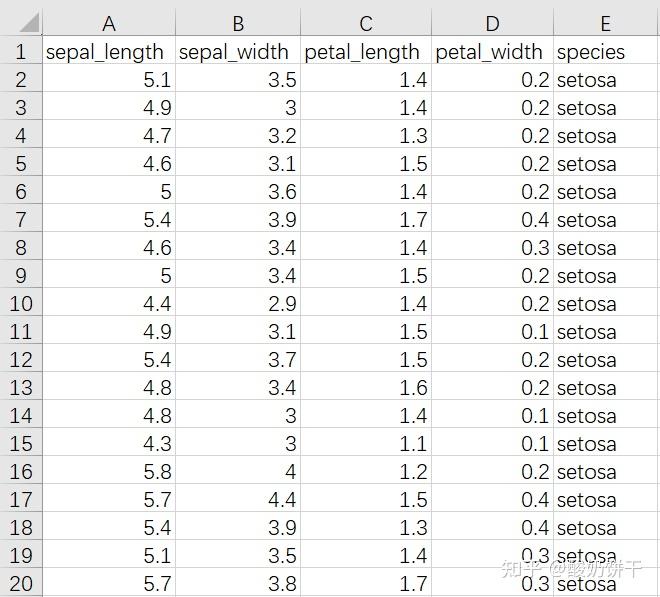
通篇以iris(鸢尾花)数据集为例
(下图为数据集部分内容)
1.如何对其进行数据处理?
从iris数据集中,提取前两个分类的数据,并以[sepal length,sepal width]作为特征,即提取iris数据集中的样品:前100个;变量:第1个,第2个,和倒数第1个。
##载入模块import pandas as pdimport numpy as npfrom sklearn.datasets import load_iris##载入数据iris = load_iris() #np的arraydf = pd.DataFrame(iris.data, columns=iris.feature_names) #弄成pd的数据框df['label'] = iris.target #再添加一列作为标签#样品:前100个取过来,变量:第1个,第2个,和倒数第1个。注意第一个下标为0。data = np.array(df.iloc[:100, [0, 1, -1]]) data2.用sklearn实现感知机
##载入相关模块import numpy as npimport pandas as pdimport matplotlib.pyplot as plt %matplotlib inlinefrom sklearn.datasets import load_irisfrom sklearn.model_selection import train_test_splitfrom collections import Counter##载入数据iris = load_iris()df = pd.DataFrame(iris.data, columns=iris.feature_names)df['label'] = iris.target df.columns = ['sepal length', 'sepal width', 'petal length', 'petal width', 'label']##提取特征和样品(取前面100个数,第一列、第二列和最后一列)data = np.array(df.iloc[:100, [0, 1, -1]]) # 最后一个特征作为标签,其他的作为特征X, y = data[:,:-1], data[:,-1] # 前者表示的是取所有行,但不包括最后一列的数据,结果是个DataFrame。后者则是取所有行最后一列对应的一列数据,结果是Series。 # 取80%作为训练,20%作为测试X_train, X_test, y_train, y_test = train_test_split(X, y, test_size=0.2) ## 载入sklearn中的感知机模块import sklearnfrom sklearn.linear_model import Perceptronclf = Perceptron(fit_intercept=True, max_iter=1000, shuffle=True) clf.fit(X_train, y_train)## 输出感知机参数print(clf.coef_)##画图# 画布大小plt.figure(figsize=(10,10))# 标题plt.rcParams['font.sans-serif']=['SimHei']plt.rcParams['axes.unicode_minus'] = Falseplt.title('鸢尾花线性数据示例')# 散点plt.scatter(data[:50, 0], data[:50, 1], c='b', label='Iris-setosa',)plt.scatter(data[50:100, 0], data[50:100, 1], c='orange', label='Iris-versicolor')# 画感知机的线x_ponits = np.arange(4, 8)y_ = -(clf.coef_[0][0]*x_ponits + clf.intercept_)/clf.coef_[0][1]plt.plot(x_ponits, y_)# 其他部分plt.legend() # 显示图例plt.grid(False) # 不显示网格plt.xlabel('sepal length')plt.ylabel('sepal width')plt.legend()3.用sklearn实现k近邻算法
##载入相关模块import numpy as npimport pandas as pdfrom sklearn.datasets import load_irisfrom sklearn.model_selection import train_test_splitfrom collections import Counter##载入数据iris = load_iris()df = pd.DataFrame(iris.data, columns=iris.feature_names)df['label'] = iris.target df.columns = ['sepal length', 'sepal width', 'petal length', 'petal width', 'label']##提取特征和样品#取前面100个数,第一列、第二列和最后一列data = np.array(df.iloc[:100, [0, 1, -1]]) #最后一个特征作为标签,其他的作为特征X, y = data[:,:-1], data[:,-1] #取80%作为训练,20%作为测试X_train, X_test, y_train, y_test = train_test_split(X, y, test_size=0.2) from sklearn.neighbors import KNeighborsClassifierclf = KNeighborsClassifier()clf.fit(X_train, y_train)## 验证算法精度clf.score(X_test, y_test)##预测某点test_point = [[a, b], [c, d]] #a/b/c/d为随机数值(你想预测的数值)clf.predict(test_point)4.用sklearn实现朴素贝叶斯
##载入相关模块import numpy as npimport pandas as pdfrom sklearn.datasets import load_irisfrom sklearn.model_selection import train_test_splitfrom collections import Counter##载入数据iris = load_iris()df = pd.DataFrame(iris.data, columns=iris.feature_names)df['label'] = iris.target df.columns = ['sepal length', 'sepal width', 'petal length', 'petal width', 'label']##提取特征和样品#取前面100个数,第一列、第二列和最后一列data = np.array(df.iloc[:100, [0, 1, -1]]) #最后一个特征作为标签,其他的作为特征X, y = data[:,:-1], data[:,-1] #取80%作为训练,20%作为测试X_train, X_test, y_train, y_test = train_test_split(X, y, test_size=0.2) ## 载入sklearn中的朴素贝叶斯分类器中的高斯朴素贝叶斯from sklearn.naive_bayes import GaussianNBclf = GaussianNB()clf.fit(X_train, y_train)## 验证算法精度clf.score(X_test, y_test)##预测某些点clf.predict([[ a, b ]]) #a/b为你想预测的数值5.决策树
##载入相关模块import numpy as npimport pandas as pdfrom sklearn.datasets import load_irisfrom sklearn.model_selection import train_test_splitfrom collections import Counter##载入数据iris = load_iris()df = pd.DataFrame(iris.data, columns=iris.feature_names)df['label'] = iris.target df.columns = ['sepal length', 'sepal width', 'petal length', 'petal width', 'label']##提取特征和样品#取前面100个数,第一列、第二列和最后一列data = np.array(df.iloc[:100, [0, 1, -1]]) #最后一个特征作为标签,其他的作为特征X, y = data[:,:-1], data[:,-1] #取80%作为训练,20%作为测试X_train, X_test, y_train, y_test = train_test_split(X, y, test_size=0.2) ## 载入sklearn中的决策树模块from sklearn.tree import DecisionTreeClassifierfrom sklearn.tree import export_graphvizimport graphvizclf = DecisionTreeClassifier()clf.fit(X_train, y_train,)## 验证算法精度clf.score(X_test, y_test)##绘制决策树tree_pic = export_graphviz(clf, out_file="mytree.pdf")with open('mytree.pdf') as f: dot_graph = f.read()graphviz.Source(dot_graph)6.逻辑回归
##载入相关模块import numpy as npimport pandas as pdimport matplotlib.pyplot as plt%matplotlib inlinefrom sklearn.datasets import load_irisfrom sklearn.model_selection import train_test_splitfrom collections import Counter##载入数据iris = load_iris()df = pd.DataFrame(iris.data, columns=iris.feature_names)df['label'] = iris.target df.columns = ['sepal length', 'sepal width', 'petal length', 'petal width', 'label']##提取特征和样品#取前面100个数,第一列、第二列和最后一列data = np.array(df.iloc[:100, [0, 1, -1]]) #最后一个特征作为标签,其他的作为特征X, y = data[:,:-1], data[:,-1] #取80%作为训练,20%作为测试X_train, X_test, y_train, y_test = train_test_split(X, y, test_size=0.2) ## 载入sklearn中的逻辑回归模块from sklearn.linear_model import LogisticRegression## 模型训练clf = LogisticRegression(max_iter=200)clf.fit(X_train, y_train)## 输出模型参数print(clf.coef_, clf.intercept_)## 验证算法精度clf.score(X_test, y_test)## 绘制x_ponits = np.arange(4, 8)y_ = -(clf.coef_[0][0]*x_ponits + clf.intercept_)/clf.coef_[0][1]plt.plot(x_ponits, y_)plt.plot(X[:50, 0], X[:50, 1], 'bo', color='blue', label='0')plt.plot(X[50:, 0], X[50:, 1], 'bo', color='orange', label='1')plt.xlabel('sepal length')plt.ylabel('sepal width')plt.legend()7.支持向量机
##载入相关模块import numpy as npimport pandas as pdfrom sklearn.datasets import load_irisfrom sklearn.model_selection import train_test_splitfrom collections import Counter##载入数据iris = load_iris()df = pd.DataFrame(iris.data, columns=iris.feature_names)df['label'] = iris.target df.columns = ['sepal length', 'sepal width', 'petal length', 'petal width', 'label']##提取特征和样品#取前面100个数,第一列、第二列和最后一列data = np.array(df.iloc[:100, [0, 1, -1]]) #最后一个特征作为标签,其他的作为特征X, y = data[:,:-1], data[:,-1] #取80%作为训练,20%作为测试X_train, X_test, y_train, y_test = train_test_split(X, y, test_size=0.2) ## 载入sklearn中的支持向量分类器模块from sklearn.svm import SVC##模型训练clf = SVC()clf.fit(X_train, y_train)## 验证算法精度clf.score(X_test, y_test)8.AdaBoost算法
##载入相关模块import numpy as npimport pandas as pdfrom sklearn.datasets import load_irisfrom sklearn.model_selection import train_test_splitfrom collections import Counter##载入数据iris = load_iris()df = pd.DataFrame(iris.data, columns=iris.feature_names)df['label'] = iris.target df.columns = ['sepal length', 'sepal width', 'petal length', 'petal width', 'label']##提取特征和样品#取前面100个数,第一列、第二列和最后一列data = np.array(df.iloc[:100, [0, 1, -1]]) #最后一个特征作为标签,其他的作为特征X, y = data[:,:-1], data[:,-1] #取80%作为训练,20%作为测试X_train, X_test, y_train, y_test = train_test_split(X, y, test_size=0.2) ## 载入sklearn中的支持向量分类器模块from sklearn.ensemble import AdaBoostClassifier##模型训练clf = AdaBoostClassifier(n_estimators=100, learning_rate=0.5)clf.fit(X_train, y_train)## 验证算法精度clf.score(X_test, y_test)9.kmeans聚类
##载入相关模块import mathimport randomimport numpy as npfrom sklearn import datasets,clusterimport matplotlib.pyplot as plt##载入数据,获得标签信息iris = load_iris()gt = iris['target'];gt## 获取属性信息data = iris['data'][:,:2]data## 载入sklearn中的kmeans聚类模块from sklearn.cluster import KMeans##模型训练kmeans = KMeans(n_clusters=3, max_iter=100).fit(data)## 得到类标签gt_labels__ = kmeans.labels_gt_labels__## 得到类中心centers__ = kmeans.cluster_centers_centers__## 绘图及可视化cat1 = data[gt_labels__ == 0]cat2 = data[gt_labels__ == 1]cat3 = data[gt_labels__ == 2]for ix, p in enumerate(centers__): plt.scatter(p[0], p[1], color='C{}'.format(ix), marker='^', edgecolor='black', s=256) plt.scatter(cat1[:,0], cat1[:,1], color='green')plt.scatter(cat2[:,0], cat2[:,1], color='red')plt.scatter(cat3[:,0], cat3[:,1], color='blue')plt.title('kmeans using sklearn with k=3')plt.xlim(4, 8)plt.ylim(1, 5)plt.show() ## 寻找K值from sklearn.cluster import KMeansloss = []for i in range(1, 10): kmeans = KMeans(n_clusters=i, max_iter=100).fit(data) loss.append(kmeans.inertia_ / len(data) / 3)plt.title('K with loss')plt.plot(range(1, 10), loss)plt.show()10.梯度下降实现感知机原理
##载入相关模块import numpy as npimport pandas as pdfrom sklearn.datasets import load_irisfrom sklearn.model_selection import train_test_splitfrom collections import Counterimport matplotlib.pyplot as plt##载入数据iris = load_iris()df = pd.DataFrame(iris.data, columns=iris.feature_names)df['label'] = iris.target df.columns = ['sepal length', 'sepal width', 'petal length', 'petal width', 'label']##提取特征和样品#取前面100个数,第一列、第二列和最后一列data = np.array(df.iloc[:100, [0, 1, -1]]) #最后一个特征作为标签,其他的作为特征X, y = data[:,:-1], data[:,-1] #取80%作为训练,20%作为测试#X_train, X_test, y_train, y_test = train_test_split(X, y, test_size=0.2)y = np.array([1 if i == 1 else -1 for i in y]) #把原本取值为0和1的y,调整成-1和1class Model: #初始化 def __init__(self): #初始化w,b和学习 self.w = np.ones(len(data[0]) - 1, dtype=np.float32) #data[0]为第一行的数据len(data[0]=3)这里取两个w权重参数 self.b = 0 self.l_rate = 0.1 #学习率为0.1 # self.data = data #定义线性函数 def lin(self, x, w, b): y = np.dot(x, w) + b return y # 随机梯度下降法 def fit(self, X_train, y_train): is_wrong = False #判断是否误分类 while not is_wrong: wrong_count = 0 for d in range(len(X_train)): #取出样例,不断迭代 X = X_train[d] y = y_train[d] if y * self.lin(X, self.w, self.b) <= 0: #根据错误的样本点不断更新w和b值 self.w = self.w + self.l_rate * (y * X) #w1=w0+rate*x*y self.b = self.b + self.l_rate * y #b1=b0+y wrong_count += 1 #角标(迭代次数—1) if wrong_count == 0: #直到误分类点为0,则跳出循环 is_wrong = True return 'Perceptron Model!' def score(self): pass##模型训练perceptron = Model() #实例化感知机perceptron.fit(X, y) #进行训练## 参数估计结果perceptron.w[0],perceptron.w[1],perceptron.b## 绘图x_points = np.linspace(4, 7, 10) #x轴的划分y_ = -(perceptron.w[0] * x_points + perceptron.b) / perceptron.w[1] plt.plot(x_points, y_)plt.plot(data[:50, 0], data[:50, 1], 'bo', color='blue', label='0')plt.plot(data[50:100, 0], data[50:100, 1], 'bo', color='orange', label='1')plt.xlabel('sepal length')plt.ylabel('sepal width')plt.legend()本文标题: 浅谈从业实训经验
本文地址: http://www.lzmy123.com/duhougan/164898.html


如果认为本文对您有所帮助请赞助本站